Executive Summary
The prevailing methodology for sizing off-grid and hybrid solar-storage systems in emerging markets relies heavily on deterministic “rule-of-thumb” calculations. While sufficient for small-scale residential applications in temperate climates, this approach is catastrophically inadequate for commercial and industrial (C&I) applications in the Middle East, Africa, and Southeast Asia.
These regions present a “Triad of Complexity”:
- Extreme Ambients: High temperatures that degrade hardware and alter efficiency curves non-linearly.
- Environmental Aggression: Extreme soiling (dust) or humidity/monsoon variances.
- Grid fragility: High Value of Lost Load (VoLL) requiring sophisticated reliability modeling.
This report transitions the reader from static, deterministic sizing to a Probabilistic Techno-Economic Framework. It demonstrates that system sizing is not merely a search for the correct kilowatt (kW) or kilowatt-hour (kWh) rating, but a strategic financial optimization exercise balancing Life Cycle Cost (LCC) against Loss of Load Probability (LOLP).
Part 1: The Deterministic Baseline Model
To understand advanced optimization, we must first define the industry-standard baseline. This “static” model is the foundation of most basic EPC proposals. It assumes average conditions and linear performance.
1.1 Calculating Design Daily Load
The baseline model begins with a deterministic energy balance.
The calculation for the total energy the system needs to generate is as follows: Design Energy (E_design) is determined by dividing the total daily user energy consumption (E_load) by the product of the inverter efficiency (η_inv) and the distribution efficiency (η_dist).
E_design: Total energy required to be generated (kWh/day).E_load: The arithmetic sum of the user’s connected loads over 24 hours.η_inv: Inverter efficiency, typically estimated at 0.90 to 0.95.η_dist: Distribution efficiency, accounting for wiring losses, typically 0.98.
1.2 Battery Bank Sizing (The Autonomy Method)
The baseline model sizes storage based on “Days of Autonomy” (DoA)—a static multiplier intended to cover sunless days.
The required battery capacity in kilowatt-hours (C_batt(kWh)) is calculated as follows: The Design Energy (E_design) is multiplied by the desired Days of Autonomy (DoA). This result is then divided by the product of the maximum allowable Depth of Discharge (DoD_max), the round-trip battery efficiency (η_batt), and the temperature de-rating factor (η_temp).
DoA: Desired days of backup (e.g., 2 or 3 days).DoD_max: Maximum allowable Depth of Discharge (e.g., 0.50 for Lead-Acid, 0.80 for Li-ion).η_batt: Round-trip battery efficiency.η_temp: A static temperature de-rating factor (often ignored or estimated at 0.95).
1.3 PV Array Sizing (The PSH Method)
The array is sized to replenish the battery and power the load within the available solar window, defined by Peak Sun Hours (PSH).
The required peak power of the PV array in kilowatt-peak (P_pv(kWp)) is calculated by multiplying the Design Energy (E_design) by a Safety Factor (SF). This product is then divided by the result of multiplying the minimum Peak Sun Hours (PSH_min) by the total system derating factor (η_sys).
PSH_min: The worst-month average insolation (kWh/m²/day).SF: Safety Factor, typically 1.1 to 1.3 to account for recharge speed.η_sys: Total system derating factor, accounting for soiling, shading, and wiring, usually 0.75 to 0.80.
Part 2: Technical Critique & Advanced Modeling (Physics Perspective)
The formulas in Part 1 are dangerous in the target regions because they treat efficiency and capacity as static constants. In the 45°C ambient heat of Riyadh or the varying cloud cover of Jakarta, these variables change dynamically.
2.1 The Thermodynamics of Photovoltaics
Using a static derate factor for temperature is insufficient for the Middle East. We must model the Nominal Operating Cell Temperature (NOCT) dynamically.
The Physics Reality:
Solar cells operate significantly hotter than the ambient air. The cell temperature (T_cell) is calculated by adding the ambient temperature (T_amb) to the product of the solar irradiance in watts per square meter (G) and a specific factor. This factor is derived by subtracting 20 from the Nominal Operating Cell Temperature (NOCT) and dividing the result by 800.
Where G is irradiance (W/m²). In a location like Dubai with an ambient temperature (T_amb) of 45°C and high irradiance (1000 W/m²), the cell temperature (T_cell) can exceed 75°C.
Advanced Sizing Adjustment:
The actual power output (P_output) is determined by multiplying the rated power (P_rated) by an adjustment factor. This factor is calculated as one plus the product of the temperature coefficient of power per degree Celsius (γ) and the difference between the actual cell temperature (T_cell) and the standard test condition temperature of 25°C.
Where γ is the temperature coefficient of power (per °C).
- Implication: A standard poly-crystalline panel (with a
γof -0.41%) loses approximately 20% of its output at noon in summer. A “static” model under-sizes the array by assuming standard test conditions (STC), leading to energy deficits during peak demand.
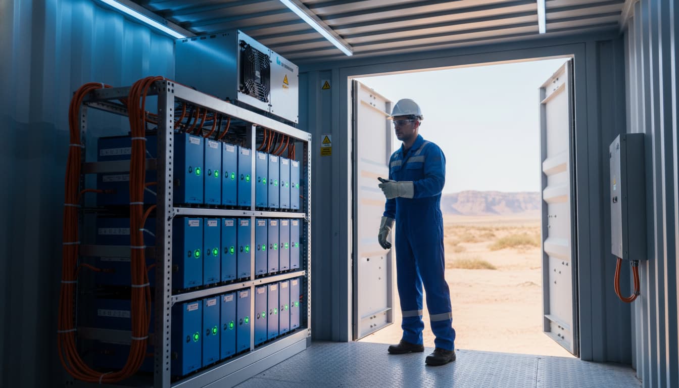
2.2 Battery Performance: The Heat/Capacity Paradox
In Part 1, we calculated the required battery capacity, C_batt. However, in sub-Saharan Africa or the Gulf, “Rated Capacity” is a theoretical number.
Thermal Degradation (Arrhenius Equation):
Battery degradation rates typically double for every 10°C rise in operating temperature.
- Lead Acid (VRLA): At 35°C, common in uncontrolled enclosures in Kenya, the useful life drops from 5 years to less than 2.5 years.
- Lithium (NMC vs. LFP): NMC chemistries suffer severe degradation and safety risks above 45°C. LFP (Lithium Iron Phosphate) is far more robust but still suffers capacity fade.
The Voltage Sag Constraint:
High temperatures increase internal resistance over time. A battery might hold the required energy (kWh), but under high load (kW), the voltage will sag below the inverter’s cutoff point prematurely.
- Design Correction: We must size for End-of-Life (EoL) power capability, not just Beginning-of-Life (BoL) energy capacity.
2.3 Environmental Loss Factors
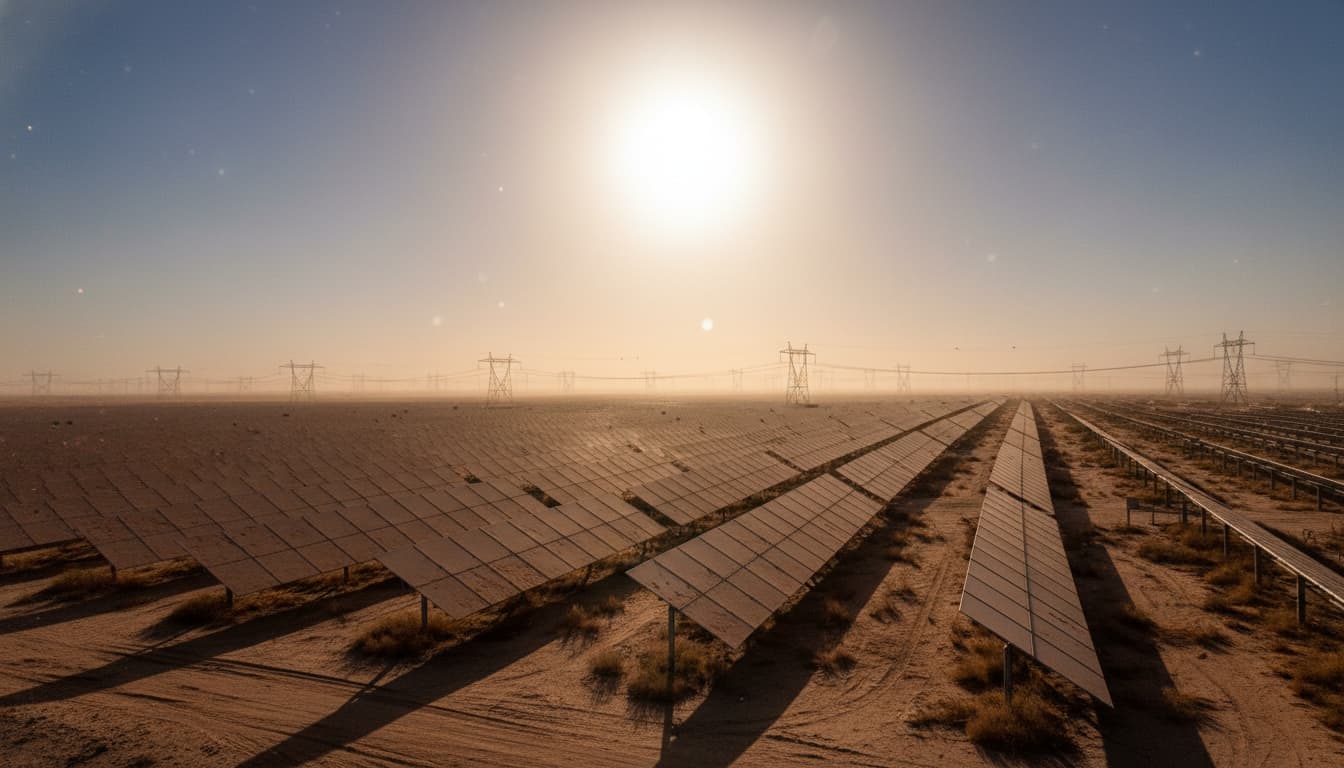
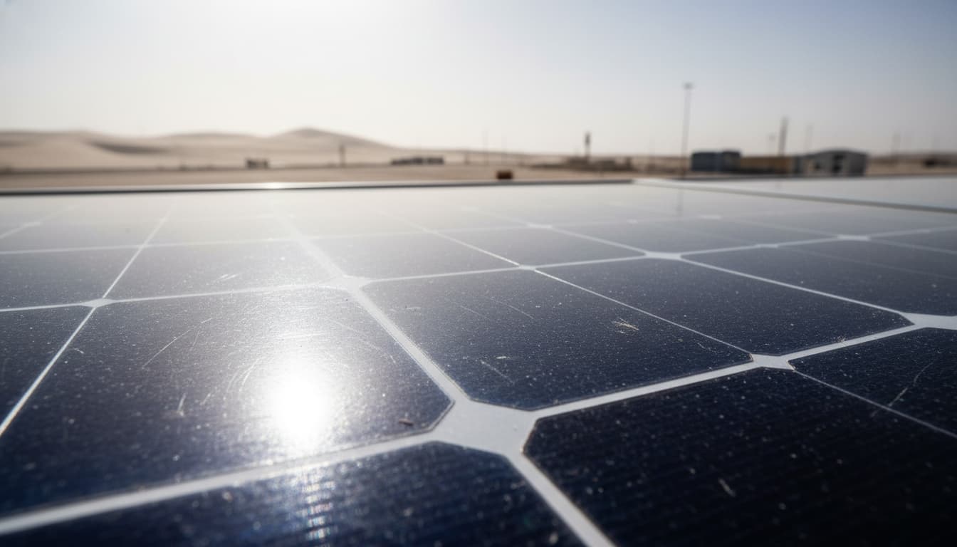
- The Middle East (Soiling): Standard derating assumes 2-3% soiling loss. In Oman or Saudi Arabia, dust accumulation can cause 0.5% loss per day. Without an automated cleaning schedule or massive oversizing (+25%), the deterministic model fails by week two.
- Southeast Asia (Humidity & Cloud Shield): In Indonesia or the Philippines, “Average PSH” is misleading due to high intermittency from cloud edge effects. This requires a higher C-rate capability in batteries to capture energy during short bursts of high irradiation.
Part 3: The Economic & Risk Overlay (Financial Perspective)
A system that never fails is infinitely expensive. Engineering constraints must be bounded by financial reality.
3.1 From “Autonomy” to “Probabilistic Reliability”
“3 Days of Autonomy” is an arbitrary metric. It does not account for the probability of four consecutive cloudy days occurring once every five years.
New Metrics:
- LOLP (Loss of Load Probability): The likelihood that the load exceeds available generation.
- LLP (Loss of Load Probability): The ratio of unserved energy to total demand, calculated as the missing kilowatt-hours divided by the required kilowatt-hours.
3.2 The Value of Lost Load (VoLL)
This is the critical financial variable. It quantifies the economic loss of a power outage.
- Low VoLL: Rural residential lighting. Sizing can be “lean,” where a high LOLP is acceptable.
- High VoLL: A telecom tower or cold storage facility in Nigeria. An outage means spoiled inventory or penalties for violating Service Level Agreements (SLAs).
- Formula: The justification for system reliability increases follows a specific principle: the increase in Capital Expenditure (
Δ CAPEX) must be less than the Value of Lost Load (VoLL) multiplied by the corresponding reduction in unserved energy (Δ E_unserved).
3.3 Life Cycle Cost (LCC) Analysis
We must evaluate the Levelized Cost of Energy (LCOE) over the project life (e.g., 20 years), not just the upfront CAPEX.
The Regional Impact on LCC:
In hot climates (MEA), the OPEX and replacement costs serve as the primary drivers of LCC.
- Scenario A (Cheap Upfront): Lead-acid batteries, minimal cooling. CAPEX: $50k. Replacements: Every 2.5 years (due to heat). Total LCC: High.
- Scenario B (Robust): LFP Batteries, Active AC Cooling, Oversized PV. CAPEX: $80k. Replacements: Year 10. Total LCC: Lower than A.
Inflation & Sensitivity:
In unstable economies (parts of Africa/SE Asia), relying on grid backup is risky due to tariff volatility. A larger solar system acts as a hedge against future diesel/grid inflation.
Part 4: The Integrated Decision Framework
To finalize the sizing, we move to a simulation-based decision matrix. We do not solve for one “correct” size; we solve for an optimized curve.
4.1 Methodology: Time-Series Simulation
Instead of using monthly averages, we define a simulation loop using hourly TMY (Typical Meteorological Year) data.
The Algorithm:
The simulation iterates through each hour, denoted as t, and performs the following steps:
- Calculate the photovoltaic (PV) production, represented as
P_pv(t), for that specific hour using the temperature-adjusted models described in Section 2.1. - Calculate the electrical load, represented as
L(t), for that hour. - Batteries absorb surplus or discharge deficit.
- Track the battery’s State of Charge, or
SoC. - If the battery’s State of Charge (
SoC) drops below the minimum allowed level (SoC_min), the system records a Loss of Load Event.
4.2 The Pareto Front: Cost vs. Reliability
By running this simulation thousands of times with different PV and battery sizes, we generate a Pareto Front graph. The X-axis represents the Life Cycle Cost (LCC) in dollars, and the Y-axis represents the percentage of Unmet Load.
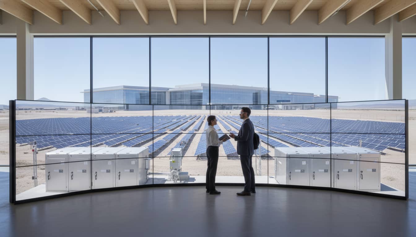
- The “Knee” of the curve represents the optimal economic design—the point where spending more money yields diminishing returns on reliability.
4.3 Regional Adaptation Strategy (Case Studies)
Case 1: The Middle East (e.g.
, Oman/UAE)
- Environment: Extreme Heat (>45°C), High Soiling.
- Sizing Strategy:
- PV: Oversize by 20-30% specifically to counter thermal losses and soiling. Use automated cleaning robots or budget for weekly cleaning. Bifacial modules are preferred due to the high albedo from sand.
- Battery: LFP Chemistry is mandatory due to better thermal safety than NMC. Batteries must be housed in an actively cooled enclosure (HVAC).
- Financials: High CAPEX due to cooling and cleaning requirements, but results in the lowest LCOE because of high solar yield.
Case 2: Sub-Saharan Africa (e.g., Rural Kenya/Nigeria)
- Environment: High logistics costs, theft risk, variable grid, and moderate heat.
- Sizing Strategy:
- PV: Employ the simplest mounting structures and theft-deterrent hardware.
- Battery: LFP is preferred for cycle life, but VRLA is often used for its lower upfront cost, which requires oversizing by a factor of two to manage the Depth of Discharge (DoD).
- Financials: The design is driven by logistics and the Value of Lost Load (VoLL). If powering a diesel-replacement microgrid, the system is sized to minimize generator runtime (Fuel Saver mode).
Case 3: Southeast Asia (e.g., Philippines/Vietnam)
- Environment: High humidity, monsoon season with extended low-light periods, and salt mist.
- Sizing Strategy:
- PV: Requires high sensitivity to cloudy-light performance, favoring Heterojunction or TopCon technologies. Mounting must be rated for typhoon wind speeds, often exceeding 200 km/h.
- Battery: A larger kWh capacity is required to ensure longer autonomy during the monsoon season, which contrasts with the predictable daily sun of the Middle East.
- Financials: High Balance of System (BoS) costs due to the need for structural wind-proofing.

Conclusion & Recommendations
For decision-makers in the Middle East, Africa, and Southeast Asia, the era of datasheet-based sizing is over. The risks of environmental degradation and the financial penalties of failure are too high.
The Strategic Checklist:
- Abandon Static Derating: Use temperature-dynamic modeling for PV yields.
- Define VoLL First: Do not ask “How much battery do I need?” Instead, ask “How much does downtime cost me?”
- Chemistry Matters: In regions where temperatures exceed 30°C, LFP is the baseline requirement. Lead-acid batteries represent a false economy.
- Simulate, Don’t Calculate: Use hourly stochastic simulations to determine the optimal trade-off between Life Cycle Cost (LCC) and reliability, often visualized as a Pareto Front.
By adopting this framework, organizations can transform energy systems from a technical cost center into a resilient, optimized financial asset.